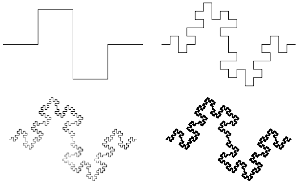
Rendering Stateless L-System in Mathematica
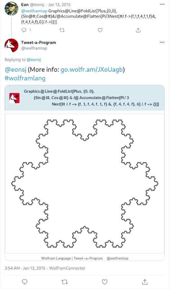
My interest in this topic was started by a code golf race started by the “Tweet-a-Program” campaign by Wolfram in 2015. Twitter limits the number of characters per tweet, so one should pull some smart tricks to cram in coolness into a tweet. Although I was not the first one nor the only one who posted fractals, I can say that, for this specific topic, my snippet was the most readable, extendible, and concise. Also, I actually learned a lot about Mathematica while doing this - much more than my few years of experience that I already had.
L-System, a.k.a Lindenmayer System, is a string rewriting system, which is often used for generating self-similar fractals. I works by iteratively applying one or more rules to the current state, starting from the initial state. If you have heard about Logo, the turtle drawing language, L-system is pretty much a recursive Logo functions.
The reason why “Stateless” is added to the title is that this post only covers non-state-aware L-systems. Some L-systems depend on save-state feature, which makes sense only in sequential state-aware interpreter. An example of such system is “Fractal Plant”. (It might be possible to simulate this behaviour by tracing back the lines, but it’s too much of work.)
Implementing L-System interpreter
The following is the code from the above tweet:
In[5]:=

Out[5]=
The most important bit here is "/."(ReplaceAll) operator. In fact, Wolfram/Mathematica language itself is a term-rewriting system, and its standard library offers pattern matching functions. That is, implementing L-system, a string rewriting system, in Wolfram language is just a matter of converting the string into a list of terms, which is far much trivial than implementing a full interpreter.
For example, Koch Snowflake can be defined like:
![]()
... and the below code applies the production rule to the initial state twice:
In[6]:=
![]()
Out[6]=

This is it. This is how we get the state of n-th level. All that’s left is rendering the final state to an actual image, which is also relatively easy using Mathematica’s symbolic graphics library.
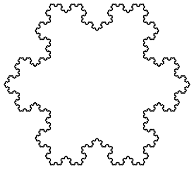
However, the code from the tweet is very limited. It assumes that every rotation(+,–) is followed by “Go Forward” symbol, which isn’t right in many cases. The end result looks like this:
In[7]:=
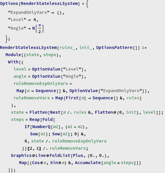
For the sake of documenting the internals, the function has 3 distinctive steps. First, it computes the target state. Second, it reforms the state into a list of rotation angles b/w lines. Notably, this step is implemented using Sow-Reap pattern. Third, draw lines based on the angles.
Below is just a utility function to simplify export and display.
In[9]:=
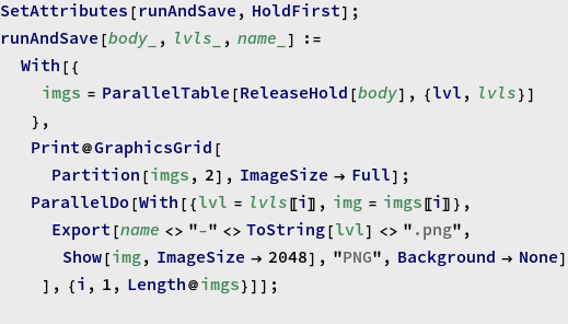
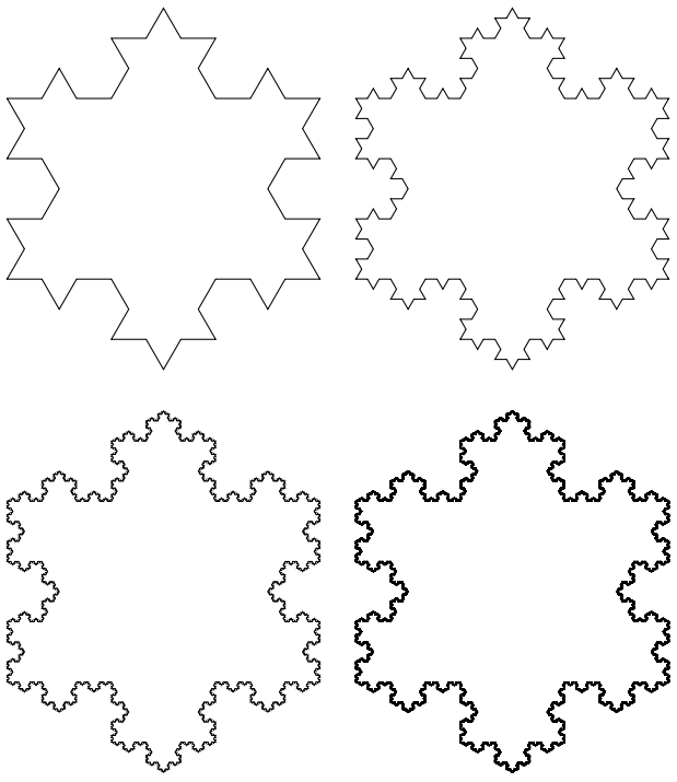
NOTE: you can find the exported image at the bottom of this page.
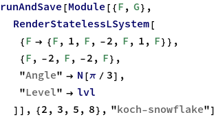
Koch Snowflake

In[11]:=
Sierpinski Triangle

In[12]:=
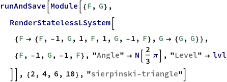
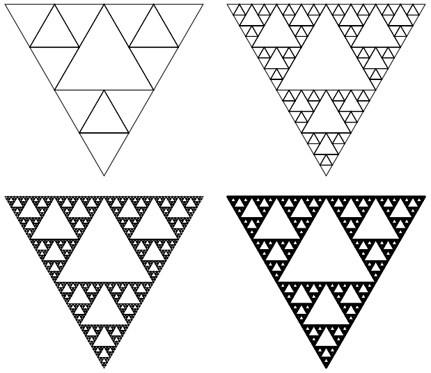
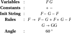
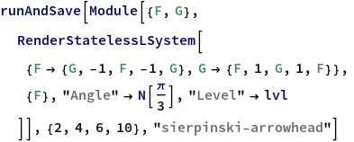
An approximation of Sierpinski Triangle using Sierpinski arrowhead curve
In[13]:=
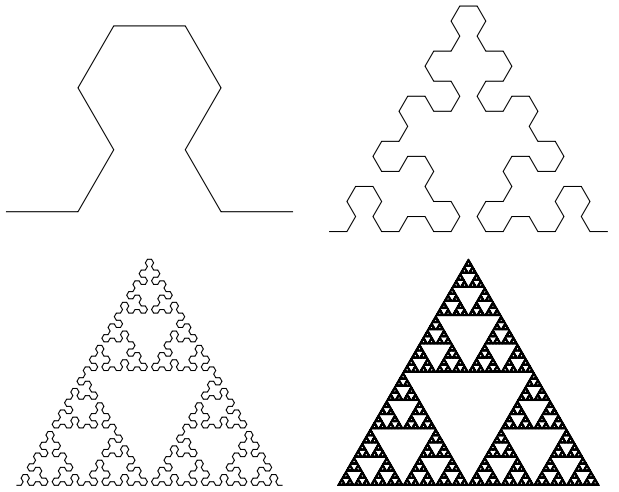
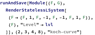
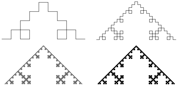
Koch Curve
In[14]:=
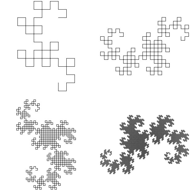
Dragon Curve
In[15]:=

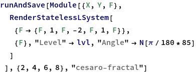
Cesàro Fractal
In[16]:=
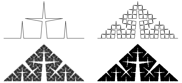
Minkowski sausage
In[17]:=

